Abstracted Modeling of Herd Immunity has been Too Oversimplified
In recent weeks, following news of the development of successful vaccines against COVID-19, conversation on herd immunity has shifted towards expectations for when normal life can be expected to resume. This is superficially in contrast to prior conversation focusing on herd immunity as something dangerous and to be avoided.
In recent weeks, following news of the development of successful vaccines against COVID-19, conversation on herd immunity has shifted towards expectations for when normal life can be expected to resume. This is superficially in contrast to prior conversation focusing on herd immunity as something dangerous and to be avoided. This contrast has, like nearly every aspect of epidemiology and especially so with herd immunity, been oversimplified.
Herd immunity is generally referred to as the concept of that a disease can stop spreading widely in a population because enough people are already immune to it — either through natural infection or vaccination. Since vaccination has emerged as an option in the future, the purported dangers of widespread proliferation of COVID-19 through natural immunity are less of a focus in establishing herd immunity moving forward.
The degree to how widespread the virus would proliferate naturally and how many (remaining) would require vaccination is often referred to as the herd immunity threshold. This single number has been established both as the outcome to avoid achieving through natural immunity and as the target to achieve in vaccination rates.
Given that recent estimates put it at 42% of Americans that will not agree to be vaccinated, that estimates for the herd immunity threshold have varied to be around 60–70% of the population required to have immunity to confer herd immunity, and that reported cases are currently at 14,146,191 and there are many (CDC estimates 11x as many) unreported cases which could represent a large portion of the U.S. population having already acquired natural immunity (which, though being one of the worst miscommunications of this crisis, does exist, and if anything like its close relatives for many years — reinfections being extremely rare and likely an artifact of how testing works), and that there may be preexisting immunity to COVID-19 from previous epidemics of other coronaviruses (which likely contributes to reduced infection and death rates in the Asia-Pacific region of the world), achieving target herd immunity rates through vaccination may be possible to some degree (especially if overlap with individuals who have tested positive previously through PCR, antigens, or antibodies is accounted for). But given the dramatic consequences of first lockdowns and the second lockdowns currently being implemented which may make those consequences even worse and prolong suffering for hundreds of millions of people being implemented to varying degrees (regardless of if lockdowns may make matters worse) and changing over time to varying degrees as those goals are met, it is important to account for sensitivity and additional complexity in those goals of herd immunity.
Past pandemics like the Black Death are still around, sometimes they can even cause multiple pandemics nearly 100 years apart — H1N1 caused both Spanish Flu (1918) and Swine Flu (2009), and sometimes widespread vaccination brings cases down very low and prevents future epidemics as in the case of Measles. No pandemic to date has been halted by a vaccine and COVID-19 is the first where that has been attempted (though it may ultimately be unnecessary in many regions to varying degrees). This begs the question — have we achieved herd immunity in the Black Death, H1N1, or even with Measles? Herd immunity is not eradication (which is itself poorly defined), and as alluded to previously, the concept of herd immunity as it is generally referred is a bit simplistic — the answer is yes, but comprehending how requires a more accurate understanding of herd immunity than has been widely reported on or otherwise discussed in the past year.
Most would be surprised, I imagine, to discover that the generally referred to concept of herd immunity does not just not mean eradication, but simply that an epidemic has peaked in new infections, and a herd immunity threshold is just where this takes place in extremely simple models. It’s actually best thought instead of stopping the spread widely in a population as just when those currently susceptible to infection are less susceptible compared to the previously susceptible population. To elaborate on this and highlight how overly simplified communication around this has been generally, it’s best to dive into the relatively simple modeling surrounding these concepts.
SIR Modeling
The SIR model is the model that has been typically used to derive understanding on the spread of infectious diseases. The model categorizes people into three groups— susceptible (S), infected (I), and recovered (R, also called removed — as it includes those for whom infection has been fatal), and can show how an epidemic may be expected to evolve over time. There are a lot of limitations to this model though, including that it treats everyone as being equally likely to be infected, equally likely to interact with other people, equally likely to transmit a virus, and that populations are constant (they are not — see H1N1, nor do any of the other limitations reflect reality) all both with respect to the individuals involved and with time. We’ll explore a bit on these limitations in a bit more detail shortly (with respect to time to keep things relatively simple), but first it is important to establish an understanding of the basics of this model.
There is an additional category of people useful in an SIR model, which is the number of people involved (N), useful for scaling things.
Given our current knowledge we can set initial values for these groups, and scale things to an abstract size population of 1.
Note: These numbers are to highlight the model itself and are not specific to the spread of COVID-19 or anything else — do not expect these to be directly applicable. Modeling reality fully is not necessary to showcase limitations in modeling or the understanding of it.

If we take a population of 10,000,000 people and decide to set 10 of them as initially infected (this cannot be zero), then the initial number of people remaining and expected to be susceptible in the population is the total population less those 10 (everyone infected or removed is no longer susceptible in this model). The number of removed initially should be set to zero initially. We can then scale these by dividing by the total population.
To describe how these values will evolve over time (t=0 in the above initial values), we need to set a few other values.
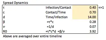
To set the overall expected number (can be thought of as a proportion) on average of susceptible individuals to be infected by a single individual who is currently infected (in a fully susceptible population) on a per unit time (daily) basis, called the effective contact rate (β — infection/time), we set the transmission rate (τ — infection/contact, since is proportion of contacts that will be infected, must be ≤1) and the contact rate (c — contact/time), and multiply the two such that β = τ*c.
To set the proportion of individuals infected who are no longer each unit of time (day) later or the removal rate (𝑣 — infection/time), we set the expected number of days on average through the entirety of the model for individuals to stay infected (d — time/infection), such that 𝑣=1/d.
The total number of individuals expected on average to become infected from a newly infected person in a fully susceptible population, called the basic reproductive number (R0 — dimensionless) is therefore defined as R0=β/𝑣=τcd.
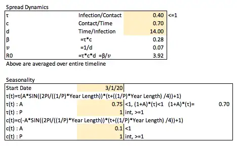
We can arbitrarily (again, this is not specific to COVID-19) set these values as follows.
These definitions allow us to describe how our population groups will change over time. The change in the susceptible population (s) would be lowered over time by the expected new infections from previous infected individuals applied to the proportion of the total population currently susceptible (working with an already scaled model this does not need to be scaled again), such that ds/dt=-βsi.
The change in the removed population (r) will be increased by the number of infected who go on to no longer be infected (this includes both recovered and dead individuals and is thus often called removed), such that dr/dt=𝑣*i.
The change in infected individuals (i) is increased by the number of individuals that are no longer susceptible, and decreased by the number of individuals that are removed, such that di/dt=(βsi)-(𝑣*i).

Given the understanding of how an SIR model works, and having set the appropriate values, we can take a look at how this model will behave.
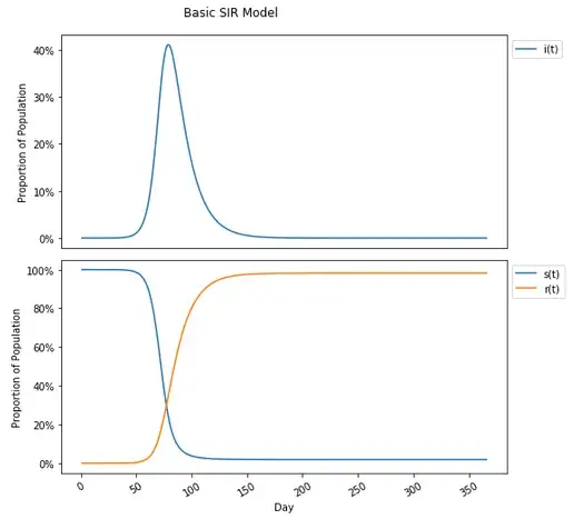
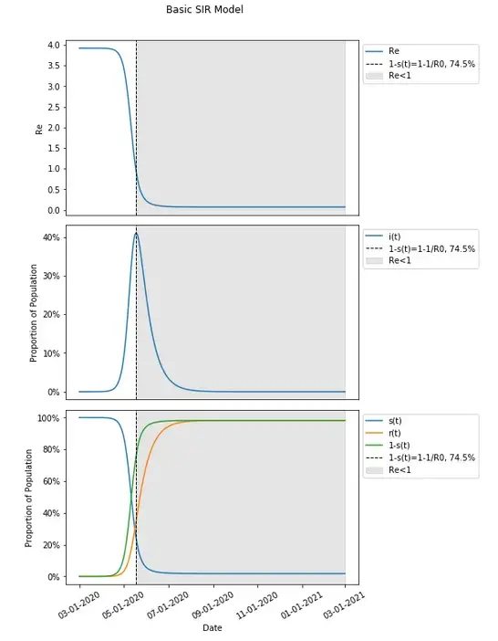
For the infected, exponential growth starts to take shape until slowing and peaking and reversing to an exponential decline. Starting with nearly 100% (100% less the initial infected amount) of the population susceptible there is an decrease over time as the virus proliferates through the population with the opposite trajectory for the removed group.
One will notice in this graph that the susceptible population plateaus to nearly zero — actually 1.8% of the population, and under the incorrect assumption that herd immunity stops the spread in the population completely, may think that the herd immunity threshold is 98.2%. This is not the case (this is actually the attack rate, which is a different concept than herd immunity, and different than eradication as well, though all have been conflated). The herd immunity threshold is defined as occurring when 1-s(t)≥1–1/R0. Given the current set values for this model, and an R0 calculated previously (from β and 𝑣) to be 3.92, that would translate to a herd immunity threshold of 1-s(t)≥1–1/R0=1–1/3.92=1–0.255=.745=74.5% which is considerably lower than the 98.2% where people no longer are getting infected. In fact placing this on the graph (along with 1-s(t), the proportion of the population not susceptible at any given point in time which includes both removed and currently infected people), this occurs much earlier, at the peak number of infections on day 79.
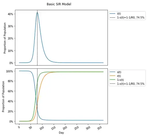
This may seem a bit confusing if one had conceived of herd immunity differently that it is defined, as I imagine many have given how many have been reporting on and discussing it. Please feel free to review other literature confirming this to be the case, but I think walking through the calculation to determine how herd immunity is defined can be useful in re-framing conceptualization of it.
Defining Herd Immunity
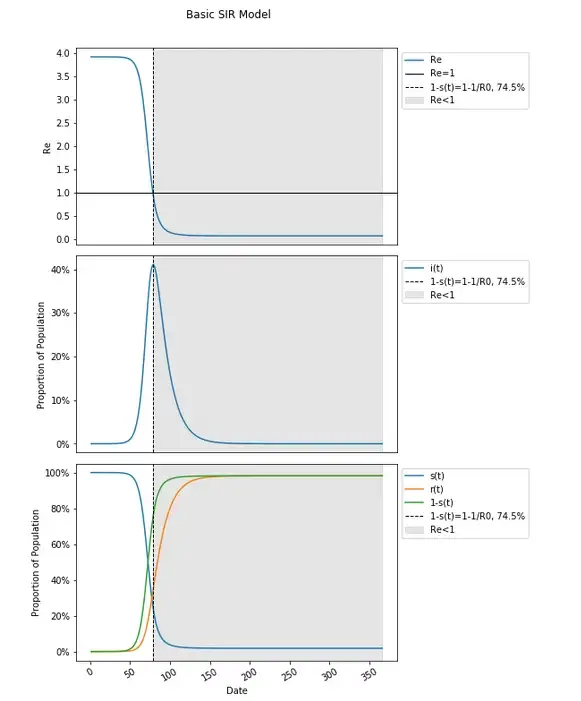
In order to determine the mathematical definition of herd immunity, it will be useful to introduce the concept of the effective reproduction rate (Re) which refers to the total number of individuals expected on average to become infected from a newly infected person in a partially susceptible population. This is similar to the basic reproductive number, but will vary over time as a result of the currently susceptible population such that Re=R0*s(t).
When enough individuals are immune in the population such that people wind up spreading the virus to less than one person on average, the spread of the virus will be endemic, and the remaining susceptible population are less likely to be newly infected compared to the previously infected population as a result of immunity in the population, this is when herd immunity takes place.
The individuals immune in the population includes those previously recovered and those currently infected in the SIR model and is equal to 1-s(t). This is sometimes referred to as pv referring to the proportion of the population that is to either be vaccinated or otherwise made immune, or pc referring to the coverage of immunity in the population. I will continue to refer to those immune as 1-s(t).
Herd immunity, therefore takes place when Re≤1 = R0*s(t)≤1 = s(t)≤1/R0 = 1-s(t)≥1–1/R0. Since this is the point at which a threshold is reached in a herd immunity threshold, we can say that the proportion of the population that needs to be immune to achieve herd immunity is at least 1–1/R0.
Including how Re changes over time and including when it hits (and remains below) one, we will find this to occur at the peak, when 1-s(t)=1–1/R0, and not during the final plateau in this graph.
The 60–70% herd immunity threshold calculations are entirely based on estimates of R0 from tracking the average number of people to whom the COVID-19 spread in presumed to be (and modeled to correct to) a fully susceptible population as places were hit early on, and insertion into the formula of 1–1/R0. These estimates for herd immunity and the resulting goals set are entirely derivative from that R0, again the average number of total people infected in a fully susceptible population by one person, has been estimated to be between 3 and 5.
It is also the case that anywhere that had hit a peak in cases (measured likely through deaths or hospitalizations, due to less and variations in widespread testing) without implementation of non-pharmaceutical interventions (NPIs) like lockdowns and others including masking (which has happened, and nine to ten months ago) that would be expected to reduce R0, have already achieved herd immunity, and potential (unclear this has been the case) reduction in post-peak cases will have occurred irrespective of that herd immunity which is again, not eradication nor the point at which no more people become infected at all.
Seasonality Introduced
Further elaborating on how a herd immunity threshold defined in an SIR model which is and has been calculated through 1–1/R0 (both in my modeling here and broadly to estimate vaccination targets and claim that natural herd immunity has not taken place in various locations) simply does not fully capture how an epidemic will continue to play out and how those goals are oversimplified and not reflective of reality, I’d like to further explore through the impact of seasonality on such models.
The reason to explore this through introducing seasonality into this model rather than heterogeneity in individuals (which has been done and on its own may result in a herd immunity threshold of 10–20%) or presumed implementation of restrictions, is that there can be simplicity in modeling seasonality through only changes things respective to time which can make it easy to showcase how simplistic herd immunity calculations do not tell much and are not useful in rebuffing that natural herd immunity has taken place at different points in time in certain locations or in setting of vaccination targets.
There is also good reason to think COVID-19 is seasonal to some degree (as are most respiratory viruses and other contagious respiratory disease).
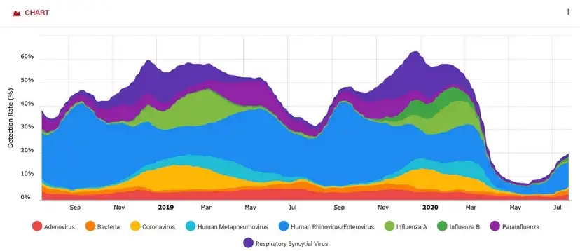
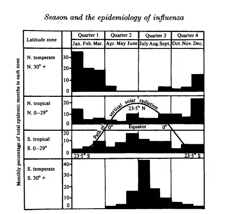
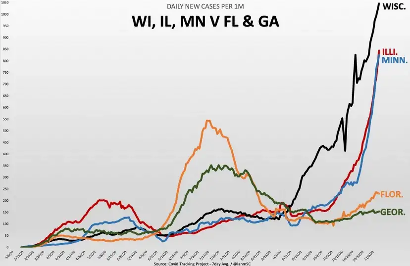
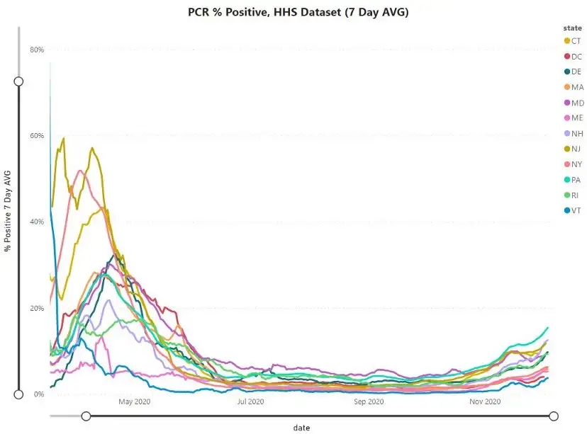
This is not the primary reasoning for introducing seasonality into this model though — as it is not meant to be directly applied to the current pandemic, but more to showcase how simple modeling applied more broadly than it should be, as the real world has a lot of complexity, can break down in meaning and fail to be useful.
In implementation of seasonality into this model, it will be useful to do a like for like comparison with the more basic model to highlight how things break down, and it will be converted to use a date instead of days, starting here at 3/1/2020 (this can and will be changed in different investigations into this model later on).
In introducing and modeling seasonality, it very well may be and likely does impact both the transmission rate (τ) and amount of contacts per unit time (c) independently. The average duration of infection (d, and therefore the removal rate, 𝑣) would not likely be impacted by seasonality.
It would be expected that cold weather would increase the transmission rate with warm weather decreasing it, and with cold weather decreasing the number of contacts a person has, and warm weather increasing the number of contacts a person has.
We can define τ at a time t (the day of the year modeled) as
τ(t)=τ*A(sin(B(t-h))+1)
A is the amplitude of the sin wave to be set (how much variation to implement) which should be less than 1 as to not have negative values for τ on any day (the +1 shifts the graph up so the set value for τ is the average value in each wave). One should also check the values set for amplitude to ensure that the set τ value when increased to the max amplitude still is ≤1 as it represents the portion of contacts that are expected to get infected.
B represents the period of the graph implemented as
B=(2PI/((1/P)*Year Length))
such that the period of the sin wave occurs P times per year which should be set as an integer number greater than or equal to one.
h represents how the graph will be shifted implemented as
h=-((1/P)*Year Length) /4
which will move the graph to the left based on the period such that the first day of the year (at 0, on 1/1 each year — arbitrarily chosen, but also does to some degree line up with seasonality in other contagious respiratory diseases, see above) will be where these values are expected to peak.
Similarly, c(t) can be defined as
c(t)=c*-A(sin(B(t-h))+1)
Focusing on differences here, the amplitude is negative for the contact rate because it is expected to have the opposite seasonal impact compared to the transmission rate with respect to how they change over time. For the contact rate, this amplitude should still be limited to be less than one (as it is multiplied by c), to not have negative values at any point in time, though as the number of contacts is not a portion of anything, the max value of c(t) does not need to be ≤1.
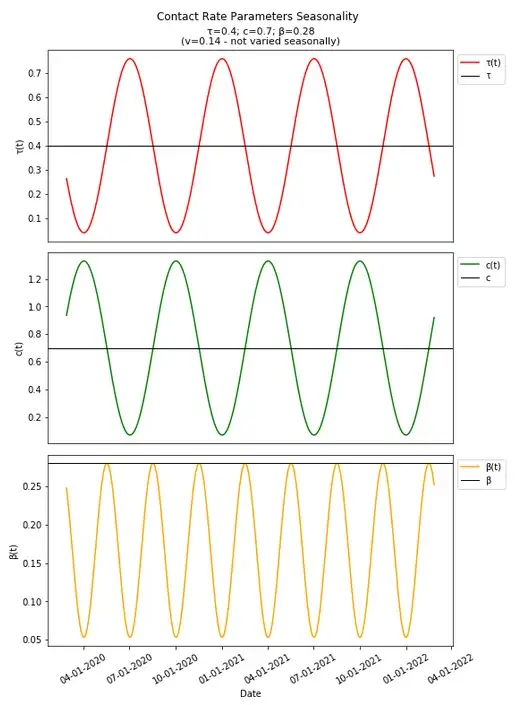
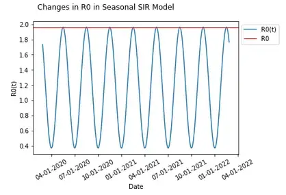
We can set these seasonality parameters arbitrarily along with an arbitrary start date (already set), and see how they along with β (and R0) change over time (R0 should be an idealized model and singly account in one non-varied value for changes over time as in the basic model if all else were equal, but the components involved in calculation of R0 do vary over time, so R0(t) is implemented, and we will explore various ways to determine an actual R0 value for calculation of herd immunity thresholds).

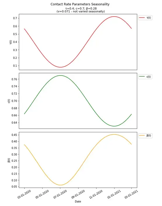
It is worth noting here that though this is meant to be simply applied just as seasonality, variations in NPIs implemented over time could impact these parameters over time in conceptually similar ways (though not likely to follow a strict sine wave solely with respect to time, again simplifying the additional complexity introduced and abstracting here).
That set variation in transmission parameters over time will be impacted by the change in susceptible population over time which can be incorporated into a simple SIR model with the same parameters established in the basic SIR model.
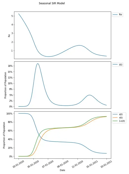
Transmission has increased sufficiently with seasonal variation that given the susceptible portion of the population resulting from that same variation in transmission dynamics, a second wave has resulted with the selected parameters.
Since these parameters are varied seasonally around the same value as in the basic SIR model, one might think of R0 as equal to the expected value in the long run, which would in this case be that same value as in the basic SIR model (and is useful in comparing the same thresholds in a basic model compared to when seasonality is introduced), and which would therefore result in a herd immunity threshold still of 74.5% We can introduce that herd immunity threshold into this graph and compare it with what we know from the basic SIR model.
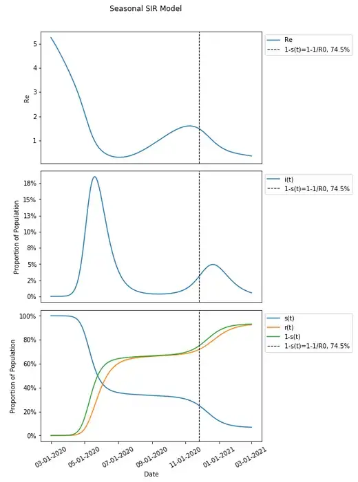
These results should be unexpected given that we would expect the remaining susceptible population to be protected from an increased risk of infection when a herd immunity threshold is reached — that had in the basic SIR model occurred at the peak of the infected population, but here, it seems that there is actually a continued increase in the population being infected after the herd immunity threshold has been reached.
In fact, we can change the seasonality parameters just slightly and produce an even more perplexing result.

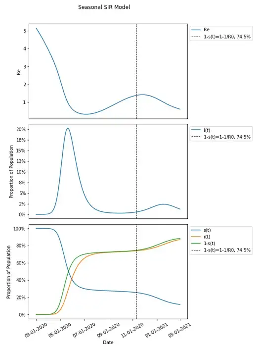
A slight change in seasonality parameters and nothing else has produced a result where the herd immunity threshold proceeds the vast majority of those infected during a second wave.
Let’s include in our graph when Re<1 to see when a person is on average expected to infect less than one person thus conferring additional protection to the susceptible population through herd immunity.
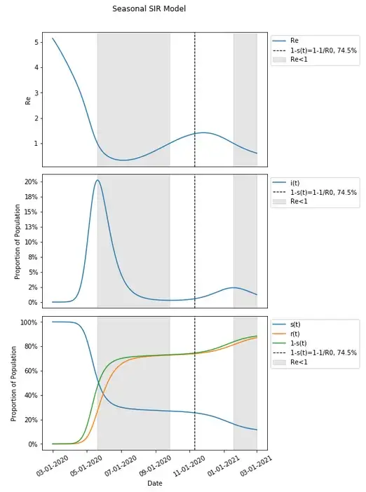
It does seem that when Re<1 aligns with the peaks in each wave when people are conferring additional protection to the susceptible population.
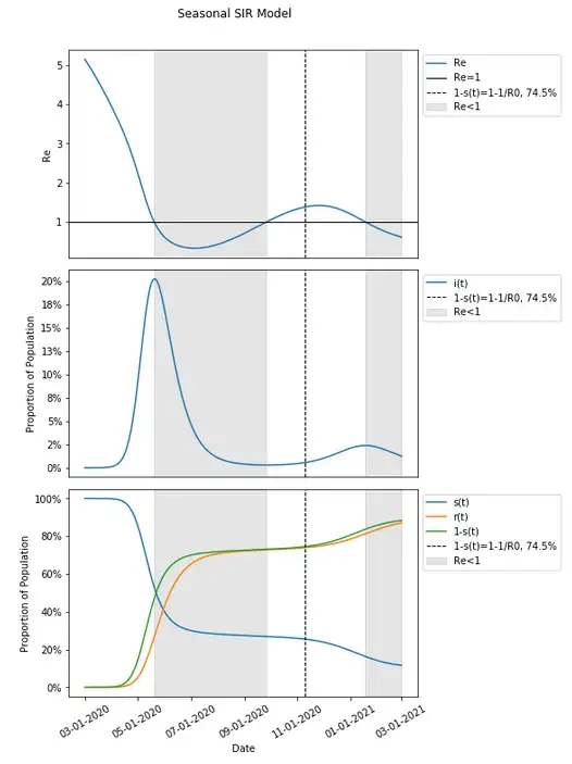
In fact, when Re<1, infections continue to get lower with additional protection conferred and when Re>1, infections continue to grow. This continues to happen in this example after 1-s(t) is past the herd immunity threshold of 74.5%.
I will posit at this point, that herd immunity is in fact not a single point where 1-s(t)>1–1/R0, but instead, whenever Re<1. This is certainly the case in a basic model where 1-s(t)>1–1/R0 is derived from when Re<1, and seems to be the case that additional protection is conferred during two separate occasions in this example of the seasonal model where 1-s(t)>1–1/R0 fails. In models with more waves (there can in fact be more than two waves even with a P of 1 for both seasonality curves, though not in this example), there will be more periods during which there is herd immunity conferred — whenever spread is epidemic and Re>1 there will not be herd immunity, and whenever spread is endemic with Re<1 herd immunity is conferred.
Variations on R0 when Varied Seasonally
Some may take that at face value, and I hope it makes sense intuitively why that proposal that herd immunity occurs whenever Re<1 would be the case. But perhaps some express concern that the misalignment of 1-s(t)>1–1/R0 and the final point where Re<1 results from that R0 is the expected average overall in a population that is fully susceptible and note that the timing of seasonality in this is irrespective of how long the epidemic lasts overall and starts at a specific point in the season. Perhaps the seasonal model has a different herd immunity threshold when given the same assumptions compared to the basic model.
If we decide arbitrarily that when the highest value for the population with immunity (1-s(t)) changes by less than 1 individual in an unscaled population of 10 million individuals is the end of the epidemic (no additional people get infected at this point, which again is not the same as herd immunity), we can take the average of R0 as it changes with seasonality (R0(t)) from day one in the model to that point to come up with a new value for R0 and calculate a herd immunity threshold from there.
When that occurs is a bit further out in time compared to our current x-axis (which has been extended below) on 2/20/2022.
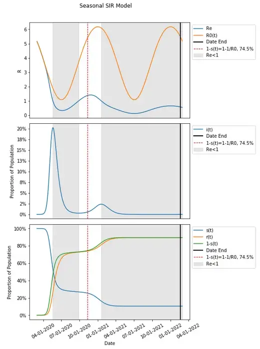
One may notice that this point where this model produces no additional people in that unscaled population becoming infected is far past the point where new cases have plateaued, and also far beyond when herd immunity (through the 1–1/R0 calculation and when the first and second periods when Re<1) has taken place.
If we average the changes in R0(t) (let’s call this R0'), the value becomes 3.75 which is actually lower than the previously determined value for R0 at 3.92. This results in a lower herd immunity threshold 73.4% compared to the 74.5% previously.
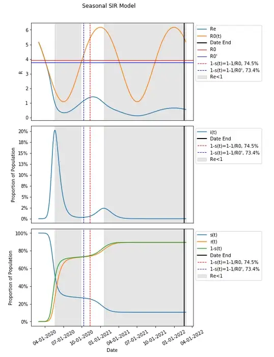
This R0' results in an even more mismatched herd immunity threshold compared to when Re<1.
One may notice that given how R0 is expected to fluctuate over time, R0' can vary in both directions.
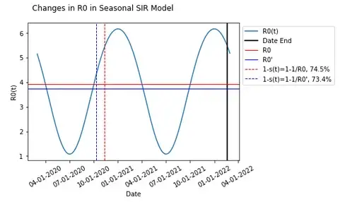
Changing the start date alone can result in an increased R0' compared to what was established by varying the date (this will also change the evolution of the epidemic as transmission dynamics vary differently over time).
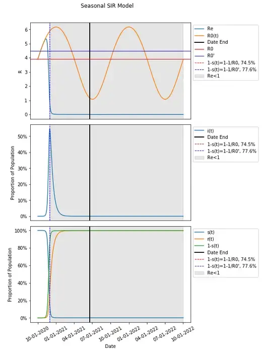
Given how this varies, it may seem like getting to a value of R0 that accounts for variation in time and may produce herd immunity that aligns with a final period of protection in the population through endemic spread may result from looking at the highest value of R0(t) as it varies.
It is worth noting here that some do attempt to describe R0 in this manner to some degree assuming that prior to restrictions the highest value of R0 would be measured — this does not account for seasonal effects described here (and in COVID-19) or other aspects of things as well, and does wind up having its own peculiarities explored here.
Returning the date in our model to 3/1/2020 (from 10/1/2020) and other spread and seasonality assumptions/parameters such that spread dynamics produce a second wave as below, we can take a look at the max value of R0(t) — we find an R0 of 6.17 and a herd immunity threshold of 83.8% (compared to 74.5%).
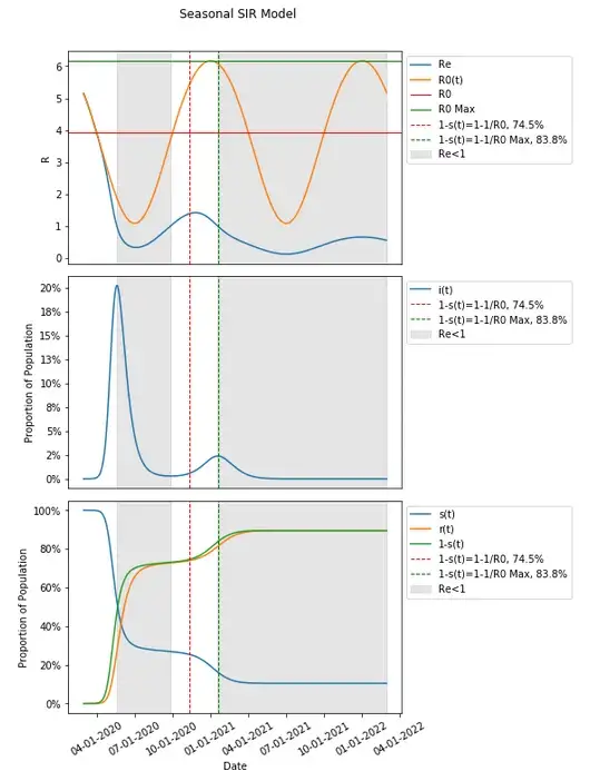
This definition of R0 does seem to align with the last period where Re<1 and the remaining population is protected by endemic spread.
Though it appears to be, 1–1/Max(R0) = 83.8% in this instance is in fact not aligned with, and does take place one day after (though this is difficult to see in the graph — highlighted values below) when Re<1 for the second time. Though it does take place afterwards and not before it seems.

That can be problematic as well though. If we change our assumptions, there is also additional complexity to this.

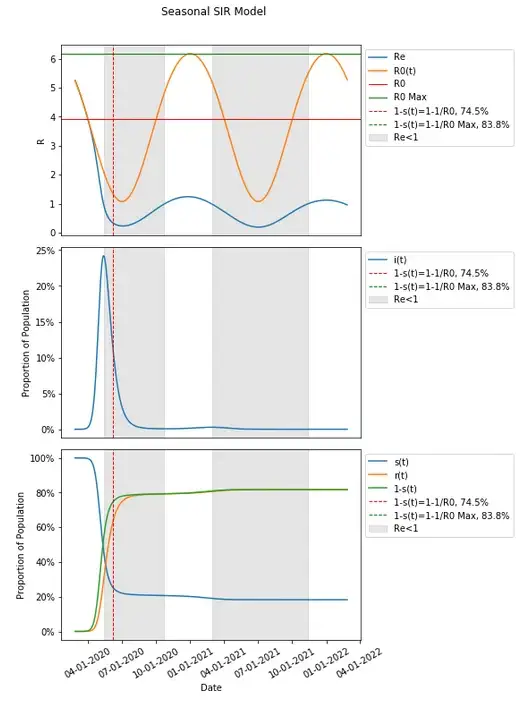
The parameters selected seem to produce a very small subsequent second and third wave — though 1–1/Max(R0) has not been reached.
Extending this out (much) further we can see many subsequent waves where there is epidemic spread and endemic spread repeating. I’ve highlighted the first two periods where Re<1, and introduced a line at Re=1 to show where that is the case for subsequent waves.
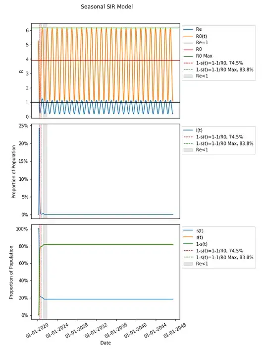
Extended out nearly thirty years the highest value for 1-s(t) is 81.7%, short of the 83.8% that would produce herd immunity with the vast majority of those infected took place very early on.
This can be exaggerated further if we change our assumptions.
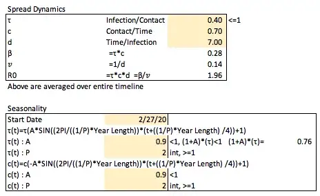
We have shown that many many waves can be produced without introducing multiple seasonality periods, but it is worth taking into account that multiple periods in our seasonality could be reflective in the real world as different regions summed together or some combination of recurring NPI impact and seasonality — again this is not meant to be realistic though. I’ve also removed R0(t) from the extended graph to highlight Re as there is significant overlap which can obscure the amount of future waves (first three are highlighted when Re<1).
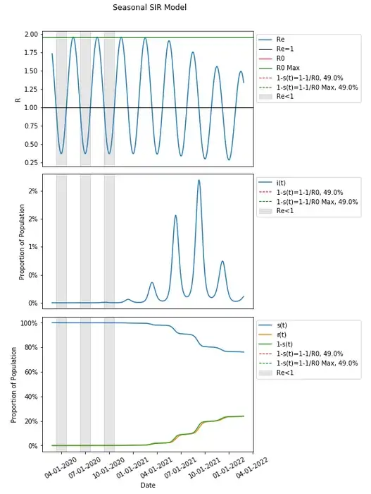
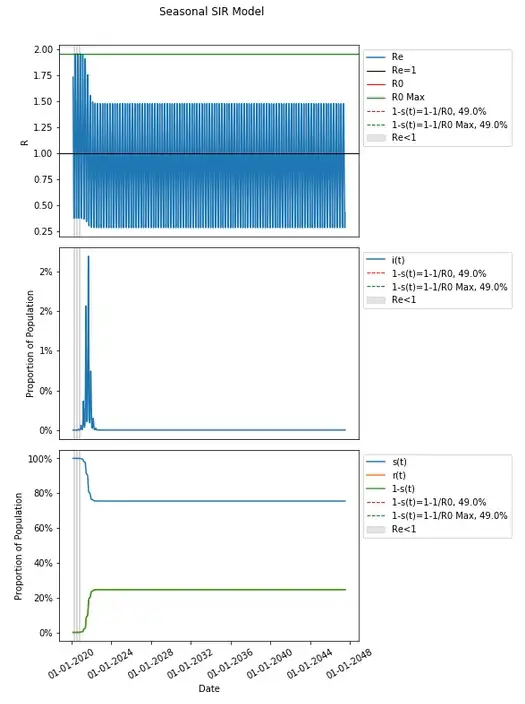
This model produces a nine large waves (a few of which are large) within the first two years and continues to have periods where spread is epidemic and endemic (as Re fluctuates above and below 1) which are relatively insignificant in their peak heights continuing for nearly thirty years and beyond.
The percentage of the population that is not susceptible, 1-s(t), does not get to any herd immunity threshold when extended this far out either — not in the original definition of R0 from the inputs, nor in R0 as the max R0 with respect to time (they are the same here — feel free to follow the calculation from assumptions and review the graphs of β and R0 over time). In fact 1-s(t) thirty years later in this model is just a hair over half that threshold of 49.0% at 24.55%.
Using Max(R0) may not be so useful either.
This is especially evident in recalling that R0 is a measure of how many will be infected by a person on average in a fully susceptible population — and Re is changes with the susceptible population. This confounding means that the only estimates of R0 that can be made are those made at t=0.
As with averaging R0 over the time until less than one person would be modeled to be infected in an unscaled population of 10 million, shifting this value in time alone will vary what the calculated herd immunity threshold is dramatically. Reverting to our earlier seasonality model assumptions and varying the date, can highlight this.

Even though R0 at t=0 is just how R0 is defined (since it is the only point where there is a fully susceptible population, though R0(t) is still useful because transmission dynamics do change over time as such) and measured (through early contact tracing), to contrast with what you would get by calculating R0 from our assumptions not varied (3.92), we will denote this R0 as R0(0). We can also compare this with the other possibilities of determining R0 (again, which are non-determinable, and do not meet the actual definition of R0) that we have already explored.
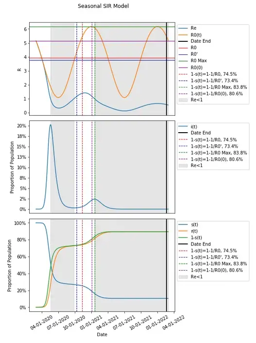
The value for R0 in this instance results in a 1–1/R0(0) calculation for a herd immunity threshold that is relatively close to that of Max(R0) (which is itself is near, but as we’ve discussed earlier with the same assumptions, occurs one day after the second and final wave in this has already hit Re<1 and peaked). This is because the where we decided to start the model falls near where that value takes place. Given how we have defined our seasonality parameters and equations, the Max(R0) falls on 1/1 each year, and the Min(R0) falls on 7/1 each year.
If we change the start date and run our model, we can observe how this impacts the herd immunity threshold (other measures of R0 and the date when 1-s(t) meets those herd immunity thresholds calculated from 1–1/R0, outside of the original calculation from assumptions will removed in these graphs to avoid clutter). It is worth noting that this will change the timing on transmission dynamics and may not result in the same wave form at all.
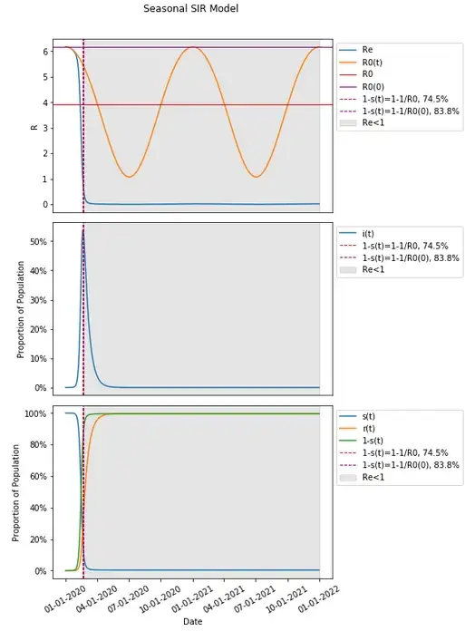
Changing the start date to 1/1/2020 results in a value for R0(0) that is high and transmission dynamics (R0(t)) that remain high in a similar time frame. This, based on our model, results in a high peaked single wave where all herd immunity threshold definitions are met. The point here though should highlight that 1–1/R0(0) is considerably higher at 83.8% than a calculated from our assumptions non-seasonal model would have at 74.5%.
This can be far lower as well if we change the start date to 7/1/2020.

Given that R0(t) hits a low of just above 1, the calculation of 1–1/R0 at R0(0) is near zero at just 7.3%, and this happens relatively easily as soon as seasonality changes transmission dynamics, resulting in a single wave. It is worth noting again that nearly 100% of the population still goes on to be infected as is the case in most scenarios (as we’ve seen this is completely divorced from the concept of herd immunity and from the calculation of a herd immunity threshold through 1–1/R0 — it can be considerably lower than that threshold, and obviously considerably higher).
A herd immunity threshold using R0(0) for the given parameters can in fact be anywhere between 7.3% and 83.8%.
Conclusions
Given the problems and variation between results in possible methods of determining R0, and that what we’ve called R0(0) is the only place to get an estimate for extrapolation (meeting the definition of R0 taking place in a fully susceptible population, where the susceptible population confounds things in real measurement of the average number of people an individual will go on to infect in a not fully susceptible population, ignoring other real world limitations in testing and contact tracing) which has served as the basis for determination of and reporting on R0 (what we’ve called R0(0)) and on herd immunity thresholds, and though an idealized R0 should account for everything which is impossible to practically determine and in itself has problems when the point 1-s(t)=1–1/R0 is never achieved as we’ve seen can be the case, 1-s(t)=1–1/R0 is ultimately both an overly simplistic and far too idealized method of determination of herd immunity.
This simple modeling can break down internally, as we’ve shown, when a single piece of complexity — seasonality — is introduced. The real world is far more complex than this. The potential degree of impact from NPI implementation, heterogeneity in transmission parameters, population differences, other regional differences, limitations in real world measurement, and yes, seasonality (which is tremendously simplified here), along with other components — all make the real world far more complex than this.
None of this is specifically to point out that NPIs may not work ultimately (though it should call into question what degree their impact has been), but rather to highlight how those reporting (incorrectly) that a place like New York City never had achieved herd immunity and enacting restrictions and vaccination goals as a result are acting on the basis of models and single number estimates of R0 directly translating to a herd immunity threshold of 60–70% that is far too simplistic and breaks down when introducing complexity, and doesn’t tell the full story of what herd immunity is at all.
1-s(t)=1–1/R0 (how it has been estimated in a fully susceptible population — what we’ve called R0(0)) is just not a good way to define herd immunity in the real world, and only is consistent in the most basic of models.
Let’s think about what herd immunity actually is supposed to be. It’s the concept of when people are protected by that others have already been exposed to or vaccinated from a disease.
As we’ve seen, infected people can and often infect dramatically more people after the point where the not susceptible population is at a rate of at least 1–1/R0 and they can continue to also infect on average more than one person. The point when few additional people are infected is not the point when non-susceptible people are protecting the remaining infected population — this is not the definition of herd immunity in 1–1/R0, nor is it what we’ve observed.
A susceptible population of people are protected when the number of non-susceptible people is such that an infected person goes on to infect less than one person. This is not a static thing as we’ve seen, and there can be periods where people are protected and where people are not; herd immunity can be had and lost (H1N1 is a clear example of where herd immunity gave way, in that case from population differences, and resulted in two pandemics). Whenever people are infecting less than one person on average (regardless of what NPIs or other factors play into that people are infecting others at that rate)— that the number of people previously infected has reduced transmission to less than one person on average for each newly infected person means that herd immunity is protecting the susceptible population, and when they are not, it is not — this determined solely by when Re<1.
It is important to note that complexity explored here that breaks the simple often incorrect projections and derivative incorrect understanding of herd immunity extends beyond one domain of additional complexity in herd immunity determinations (heterogeneity in populations can result in a herd immunity threshold of 10–20%) and more broadly in modeling every aspect of the evolution of this pandemic the resulting consequences and potential of various strategies. The real world is not so simple as to be described as by estimates of a single number in an extremely simple formula.
All of the additional complexity introduced into herd immunity determinations extends to other things — testing rates and prioritization in testing, distributions and heterogeneity of the proportion of those infected who tested positive, varying rates of positives that are false, distributions and heterogeneity of various populations in death and hospitalization rates, the degree of coincidental timing of NPI implementation with other components of impacting spread dynamics, and heterogeneity in NPI implementation — all are among what in the real world adds complexity that has rarely been accounted for to any degree in much of the scientific and political discourse and the reporting on this crisis. They should impact that discourse more broadly than they have given how expectations can be changed by incorporating that additional complexity as we’ve demonstrated.
Assuming adverse outcomes have been averted by the continuation of NPIs like lockdowns among other restrictions which can be draconian and adversely impact many people in many ways (likely more than projected potential consequences were they not in place) and are set to continue to varying degrees until set goals are met, all on the basis of overly simplistic models, is ultimately a failure in understanding complexity in the real world resulting in breaking and continuing to break society, perhaps (likely in my opinion) in completely unnecessary ways, and in holding us back from beginning to rebuild.
